Explore our expert-made templates & start with the right one for you.
Table of contents
Cloud data warehouses (CDWs) store and process different types of data to deliver value to the business. Whereas storage and compute were previously tightly coupled, modern platforms have separated them for better scalability.
While this evolution in analytics platforms has been great for migrating batch workloads of structured data to the cloud, an increasing proportion of workloads need to occur in near real time and operate on semi-structured data. This report evaluates the performance and cost of several methods for performing up to the minute processing on semi-structured data, using Snowflake Data Platform as the destination.
Introduction
The advent of the cloud data warehouse (CDW) including Amazon Redshift, Snowflake, Google BigQuery and Azure Synapse Analytics has kicked off a migration of BI reporting and analytics to the cloud, primarily off-loading or replacing the on-prem data warehouse for handling structured batch data. Naturally companies who have adopted a CDW want to leverage that investment to their big data and streaming data. The question is whether the CDW offers sufficiently low latency and price/performance to do the job.
Upsolver is a data transformation engine, built for data lakes, that automates complex orchestrations with SQL-based declarative pipelines. Upsolver customers deal with complex data sets, such as machine generated data, whether structured or semi-structured, that is continuously arriving as streams or small, scheduled batches. They rely on both data lakes and data warehouses in their architecture and have both internal and external data consumption use cases. So we often get asked, “What is the best way to architect our infrastructure for the future?”
This benchmark report reviews four approaches to processing data for near real-time analytics, using Snowflake Data Platform as the destination for analytics. Our goal was to understand the differences and trade-offs across these requirements:
- Latency to obtain query-ready data
- Cloud compute cost to process the data
- Time required to develop and maintain the data pipeline
- Cost and complexity of infrastructure the data team needs to maintain as scale, velocity and consumption requirements change
What Did We Test and Why?
This benchmark is designed to test continuous ingestion and processing of data. We chose a data set that would match what our customers see in the real world. To that end, we used a semi-structured retail order data set consisting of 16,634,450,654 records representing 5 days of continuously flowing data. This equates to 6.9 GB per hour and 840 GB in total total. The data arrives in a nested JSON file format
In order to measure the cost of updating an existing destination table on a continuous basis, we loaded 5 days of data into the destination system to create our three target tables, and then measured the time and cost of ingesting incremental data and updating aggregated values in the target tables. We evaluated two scenarios, one where new data is served each minute, and another where it is served hourly.
We measured the following:
- Cost of compute for ingesting the data and running the transformation
- Time to ingest and process the data
- Time to develop the transformation pipeline
(We considered using the TPC-DI data set, but chose not to as it was designed to simulate batch, structured workloads. It also has not been updated since 2014.)
The Four Methods We Compared
We focused on methods that our customers and solution integrator partners would commonly consider in order to achieve the best results, namely:
- Upsolver to Snowflake: Data is ingested and processed by Upsolver before being merged into a Snowflake query-ready target table.
- Snowflake Merge Command: The new data is matched with historical data in the Snowflake staging area and then merged into the existing table targets.
- Snowflake Temporary Tables: The new data is aggregated into a new temporary table before replacing the current production table, after a merge, and after deleting the old table.
- Snowflake Materialized Views: Snowflake native functionality that allows customers to build pre-computed data sets that can improve query performance, but can impact processing time and cost.
We considered a potential 5th option: A lambda architecture where an aggregate would be created via a historical table with a current view table. While this is a viable option, it requires complex orchestration configuration, duplicative logic/code, and limits the ability to update the table. We felt the complexity and overhead of this option would outweigh any potential benefits. Therefore we excluded it from consideration.
Data Warehouse and Upsolver Configurations
- Upsolver: Configuring Upsolver is straightforward. With Upsolver, you choose the number of cores you would like and set auto-scale limits for handling bursts. For this benchmark we used one AWS instance of Upsolver (4 cores) which is the smallest cluster offered.
- Snowflake: There is little required to configure with Snowflake. You only have to choose the virtual data warehouse size and the service tier you will be leveraging. We chose a size L virtual data warehouse for this test.
| System | Cluster | Cost / Hour |
| Upsolver | 4 cores | $3.50/unit per hour with a $12,600k/year minimum |
| Snowflake | Large Virtual Data Warehouse | $32/hour ($4/credit @ 8 credits/hour) |
Snowflake cost is based on the “Business Critical” service tier. We chose Business Critical as we assumed companies would need to ensure secure data access of critical streaming datasets, which the other tiers lack. If you use a lower service tier, your costs would be 25% (Enterprise tier) or 50% (Standard tier) lower.
Method 1: Upsolver to Snowflake
Step 1: Ingestion
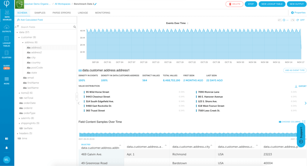
In order to ingest data with Upsolver, you connect Upsolver to an S3 bucket using the built-in AWS S3 Connector. Once connected, Upsolver reads the data and auto-generates the schema, including nested JSON files. This means you avoid the time required to inspect the data. Also, Upsolver automatically flattens nested data.
Step 2: Create Outputs for Each Aggregation
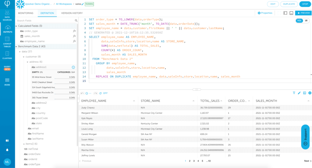
Once the schema is available to read, you create Snowflake outputs and write a single SQL statement for each of the three output tables. Since Upsolver is a declarative pipeline system, you do not need to orchestrate and manage a directed acyclic graph (DAG) in order to generate the tables. 3rd-party orchestration tools like Airflow or dbt are not needed. You can “Preview” and then “Run” the pipeline to set it in motion.
Developing this pipeline took roughly 2 hours.
Methods 2, 3 and 4: Ingest and process in Snowflake
You first load the data into Snowflake, which requires the following steps for semi-structured files like JSON.
Step 1: Copy
First you copy raw data into a single VARIANT column table. This allows the data to remain nested without alteration.
Create or replace TABLE RAW_ORDERS(
  SRC VARIANT
);

copy into RAW_ORDERS
from @MEISNOW FILE_FORMAT = ( TYPE = "JSON" );
Step 2: Flatten
Second, you map out the nested data and the required data types in order to move the data into a flattened table.
create or replace TABLE stg_orders_fd (
    CUSTOMER_ADDRESS_ADDRESS1 VARCHAR(16777216),
    CUSTOMER_ADDRESS_ADDRESS2 VARCHAR(16777216),
    CUSTOMER_ADDRESS_CITY VARCHAR(16777216),
    CUSTOMER_ADDRESS_COUNTRY VARCHAR(16777216),
    CUSTOMER_ADDRESS_POSTCODE VARCHAR(16777216),
    CUSTOMER_ADDRESS_STATE VARCHAR(16777216),
    CUSTOMER_EMAIL VARCHAR(16777216),
    CUSTOMER_FIRSTNAME VARCHAR(16777216),
    CUSTOMER_LASTNAME VARCHAR(16777216),
    DATA_DATA_ITEMS_CATEGORY VARCHAR(16777216),
    DATA_DATA_ITEMS_DISCOUNTRATE FLOAT,
    DATA_DATA_ITEMS_ITEMID FLOAT,
    DATA_DATA_ITEMS_NAME VARCHAR(16777216),
    DATA_DATA_ITEMS_QUANTITY FLOAT,
    DATA_DATA_ITEMS_UNITPRICE FLOAT,
    NETTOTAL FLOAT,
    ORDERDATE TIMESTAMP,
    ORDERID VARCHAR(16777216),
    ORDERTYPE VARCHAR(16777216),
    SALEINFO_SOURCE VARCHAR(16777216),
    SALEINFO_STORE_LOCATION_COUNTRY VARCHAR(16777216),
    SALEINFO_STORE_LOCATION_NAME VARCHAR(16777216),
    SALEINFO_STORE_SERVICEDBY_EMPLOYEEID FLOAT,
    SALEINFO_STORE_SERVICEDBY_FIRSTNAME VARCHAR(16777216),
    SALEINFO_STORE_SERVICEDBY_LASTNAME VARCHAR(16777216),
    SALEINFO_WEB_IP VARCHAR(16777216),
    SALEINFO_WEB_USERAGENT VARCHAR(16777216),
    SHIPPINGINFO_ADDRESS_ADDRESS1 VARCHAR(16777216),
    SHIPPINGINFO_ADDRESS_ADDRESS2 VARCHAR(16777216),
    SHIPPINGINFO_ADDRESS_CITY VARCHAR(16777216),
    SHIPPINGINFO_ADDRESS_COUNTRY VARCHAR(16777216),
    SHIPPINGINFO_ADDRESS_POSTCODE VARCHAR(16777216),
    SHIPPINGINFO_ADDRESS_STATE VARCHAR(16777216),
    SHIPPINGINFO_METHOD VARCHAR(16777216),
    SHIPPINGINFO_RECIPIENT_FIRSTNAME VARCHAR(16777216),
    SHIPPINGINFO_RECIPIENT_LASTNAME VARCHAR(16777216),
    TAXRATE FLOAT
);
Step 3: Insert
Third, you INSERT data from the raw JSON format into the flattened table, after mapping each object to the table.
INSERT INTO stg_orders_fd
SELECT
src:customer.address.address1::string as CUSTOMER_ADDRESS_ADDRESS1,
src:customer.address.address2::string as CUSTOMER_ADDRESS_ADDRESS2,
src:customer.address.city::string as CUSTOMER_ADDRESS_CITY,
src:customer.address.country::string as CUSTOMER_ADDRESS_COUNTRY,
src:customer.address.postCode::string as CUSTOMER_ADDRESS_POSTCODE,
src:customer.address.state::string as CUSTOMER_ADDRESS_STATE,
src:customer.email::string as CUSTOMER_EMAIL,
src:customer.firstName::string as CUSTOMER_FIRSTNAME,
src:customer.lastName::string as CUSTOMER_LASTNAME,

    itemdata.value:category as "DATA_DATA_ITEMS_CATEGORY",
    itemdata.value:discountRate as "DATA_DATA_ITEMS_DISCOUNTRATE",
    itemdata.value:itemId as "DATA_DATA_ITEMS_ITEMID",
    itemdata.value:name as "DATA_DATA_ITEMS_NAME",
    itemdata.value:quantity as "DATA_DATA_ITEMS_QUANTITY",
    itemdata.value:unitPrice as "DATA_DATA_ITEMS_UNITPRICE",

src:netTotal::float as NETTOTAL,
src:orderDate::TIMESTAMP as ORDERDATE,
src:orderId::string as ORDERID,
src:orderType::string as ORDERTYPE,

src:saleInfo.source::string as SALEINFO_SOURCE,
src:saleInfo.store.location.country::string as SALEINFO_STORE_LOCATION_COUNTRY,
src:saleInfo.store.location.name::string as SALEINFO_STORE_LOCATION_NAME,
src:saleInfo.store.servicedBy.employeeId::string as SALEINFO_STORE_SERVICEDBY_EMPLOYEEID,
src:saleInfo.store.servicedBy.firstName::string as SALEINFO_STORE_SERVICEDBY_FIRSTNAME,
src:saleInfo.store.servicedBy.lastName::string as SALEINFO_STORE_SERVICEDBY_LASTNAME,
src:saleInfo.web.ip::string as SALEINFO_WEB_IP,
src:saleInfo.web.userAgent::string as SALEINFO_WEB_USERAGENT,

src:shippingInfo.address.address1::string as SHIPPINGINFO_ADDRESS_ADDRESS1,
src:shippingInfo.address.address2::string as SHIPPINGINFO_ADDRESS_ADDRESS2,
src:shippingInfo.address.city::string as SHIPPINGINFO_ADDRESS_CITY,
src:shippingInfo.address.country::string as SHIPPINGINFO_ADDRESS_COUNTRY,
src:shippingInfo.address.postCode::string as SHIPPINGINFO_ADDRESS_POSTCODE,
src:shippingInfo.address.state::string as SHIPPINGINFO_ADDRESS_STATE,
src:shippingInfo.method::string as SHIPPINGINFO_METHOD,
src:shippingInfo.recipient.firstName as SHIPPINGINFO_RECIPIENT_FIRSTNAME,
src:shippingInfo.recipient.lastName as SHIPPINGINFO_RECIPIENT_LASTNAME,
src:taxRate::float as TAXRATE
    from RAW_ORDERS raw_source,
    LATERAL FLATTEN( input => raw_source.src:data, outer => true, path =>'items') as itemdata
You now have a workable output data set. This process took 15 hours to build, which included the time it took to extract the schema from the raw nested data, write the shell script to run the pipeline jobs and define and fine-tune the transformations using optimizations such as clustering and ordering on the tables.
Since workflows can and do change regularly, data engineers may find that they spend substantial time configuring these steps and then orchestrating them using a system like Airflow or dbt. Once a pipeline is in production, even a small change to the schema or transformation logic can require several hours of work to update, test and deploy.
Step 4: Begin Testing
Now that the data has been properly prepared, you can aggregate the data using each of the three methods. The code used for performing the merge, temporary table, and materialized view aggregation strategies can be found in the appendix.
Results
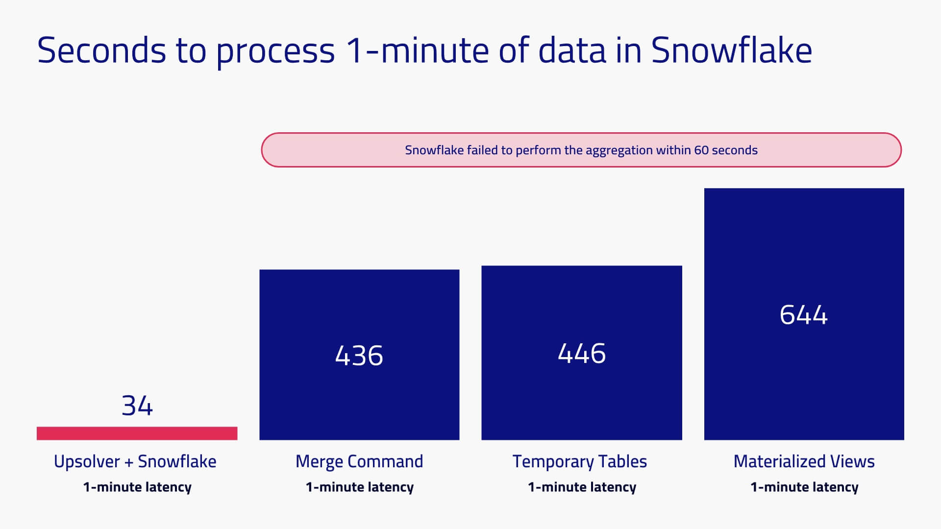
We measured the processing time and the cost of each method. Our initial intention was to only measure one minute increments but we had to also test hourly loads once we discovered that Snowflake couldn’t process the per-minute data fast enough.
Goal: 1-minute latency
In this test we pre-loaded all 5 days of data into Snowflake and reserved one minute of data to be processed for the test. Upsolver took 34 seconds to ingest and process one minute of data. Snowflake took anywhere from 436 to 654 seconds (7 to 11 minutes), which of course is outside the required window.
Goal: 1-hour latency
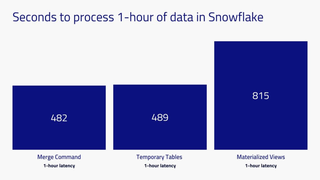
In this test we pre-loaded all 5 days of data into Snowflake and reserved one hour of data to be processed for the test. Snowflake processing time ranged from 482 to 815 seconds (8 to 14 minutes) to process one hour of data, depending on the method. It only took marginally longer to process 60 minutes of data than one minute of data, because the longest part of the entire process is the time required to scan the historical records.
The cost of each workload was calculated as followed:
Upsolver: The cost of purchasing one unit of Upsolver via AWS Marketplace is $12,600/year. As it turns out, for this specific test, we only utilized 30% of a 4-node cluster (1 Upsolver unit).
Snowflake: The advertised rate for Snowflake Business Critical Edition is $4/credit and a Large virtual data warehouse costs 8 credits/hour, for a total hourly cost of $32.
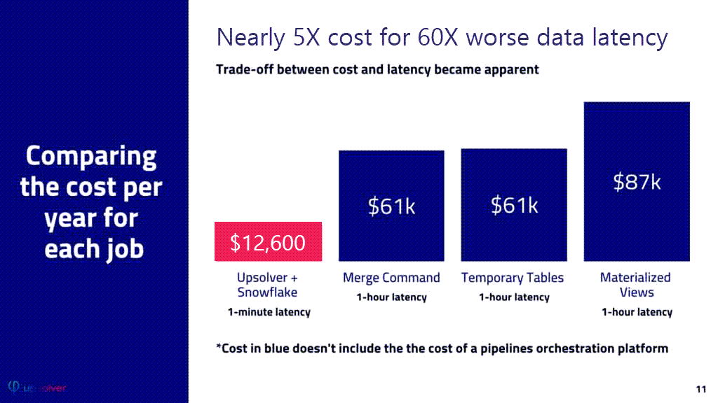
Since the performance for per-minute data load was too long to be feasible on Snowflake, we only compared costs for the Upsolver’s 1 minute latency scenario vs. the three Snowflake 1-hour latency scenarios. Using Upsolver to ingest and process the data turned out to be 70% to 81% less expensive than performing those operations in Snowflake.
Here is how we calculated the cost for Materialized Views:
Conclusions
We were unable to achieve 1-minute latency with a Snowflake Large virtual data warehouse without first processing the data using Upsolver. It is conceivable we could have achieved sub-minute latency by choosing a larger Snowflake virtual warehouse, but this would also make the processing cost prohibitive. If we assume performance scales linearly, then moving to a 4XL size virtual data warehouse would bring latency to under a minute. The 815 seconds observed for Materialized Views would be reduced to 51 seconds but cost you over $4,400,000 a year! You could avoid this cost by adopting a lambda architecture, but then would take on substantial pipeline complexity.
While a one hour latency was achievable with Snowflake, the overall costs for running the job was roughly 5X higher than processing the data using Upsolver.
These results are not particularly surprising. Snowflake was built to process end-user analytics queries on batch data, whereas Upsolver is built for data ingestion and processing of large amounts of complex and continuous data. Pairing them together in a best-of-breed coupling would be expected to provide the best results.
Lastly, there was 7.5X more data engineering work (15 hours vs. 2 hours) required to build these simple pipelines in Snowflake compared to using Upsolver. Essentially this was an extra person day per pipeline, which doesn’t scale well across hundreds of pipelines at a large organization.
Plus, Snowflake requires the implementation of an orchestration tool, which adds cost, complexity and a need for specialized skills. These costs don’t just accrue at initial pipeline design time, but accumulate throughout the lifecycle of the pipeline as maintenance issues and new requirements are addressed.
In conclusion, if you need low-latency and affordability, our testing indicates your best approach from a price, performance and time-to-develop standpoint is to use Upsolver to ingest, continuously process and serve data to your data warehouse.
Appendix 1: SQL Snippets
Upsolver SQL Pipelines
//  geo performance table
SET partition_date = DATE_TRUNC('day', TO_DATE(data.orderDate));
SET processing_time = UNIX_EPOCH_TO_DATE(time);
SELECT data.customer.address.city AS ORDER_CITY,
       data.customer.address.state AS ORDER_STATE,
       SUM(data.netTotal) AS TOTAL_SALES,
       COUNT(*) AS ORDER_COUNT,
       AVG(data.netTotal) AS AVERAGE_ORDER,
       partition_date AS ORDER_DATE
  FROM "Benchmark Data 2"
    GROUP BY data.customer.address.city,
          data.customer.address.state,
          partition_date
    REPLACE ON DUPLICATE data.customer.address.city, data.customer.address.state, partition_date
//  item performance table
SET item_category = SPLIT('|', data.items[].category);
SET order_date = DATE_TRUNC('day', TO_DATE(data.orderDate));
SET ITEM_GROUP = ELEMENT_AT(0, item_category[]);
SET ITEM_SUBCATEGORY = ELEMENT_AT(1, item_category[]);
SELECT ITEM_GROUP AS ITEM_GROUP,
       ITEM_SUBCATEGORY AS ITEM_SUBCATEGORY,
       data.items[].name AS ITEM_NAME,
       data.items[].itemId AS ITEM_ID,
       AVG(data.items[].unitPrice) AS ITEM_PRICE,
       COUNT(*) AS ORDER_COUNT,
       SUM(data.items[].quantity) AS TOTAL_ITEM_QUANTITY,
       SUM(data.items[].quantity * data.items[].unitPrice) AS ITEM_REVENUE,
       order_date AS ORDER_DATE
  FROM "Benchmark Data 2"
    GROUP BY data.items[].itemId,
          ITEM_GROUP,
          ITEM_SUBCATEGORY,
          data.items[].name,
          order_date
    REPLACE ON DUPLICATE data.items[].itemId, order_date
//  sales performance table
SET order_type = TO_LOWER(data.orderType);
SET sales_month = DATE_TRUNC('month', TO_DATE(data.orderDate));
SET employee_name = data.customer.firstName || ' ' || data.customer.lastName;
SELECT employee_name AS EMPLOYEE_NAME,
       data.saleInfo.store.location.name AS STORE_NAME,
       SUM(data.netTotal) AS TOTAL_SALES,
       COUNT(*) AS ORDER_COUNT,
       sales_month AS SALES_MONTH
  FROM "Benchmark Data 2"
    GROUP BY employee_name,
          data.saleInfo.store.location.name,
          sales_month
    REPLACE ON DUPLICATE employee_name, data.saleInfo.store.location.name, sales_month
Materialized View
create materialized view TEST.PUBLIC.MV_RPT_GEO_PERFORMANCE as
 SELECT  customer_address_city AS order_city,
       customer_address_state  AS order_state,
       SUM(netTotal)   AS total_sales,
       COUNT(*)  AS order_count,
       AVG(netTotal) AS average_order,
      DATE_TRUNC('day', TO_DATE(orderDate)) AS order_date,
      orders.orderdate
 FROM stg_orders_fd orders
   GROUP BY customer_address_city,
         customer_address_state,
        orders.orderdate;

create materialized view TEST.PUBLIC.MV_RPT_SALES_PERFORMANCE as
SELECT
  CONCAT(customer_firstName, ' ', customer_lastName)  AS employee_name,
  saleInfo_store_location_name  AS store_name,
  SUM(netTotal)  AS total_sales,
  COUNT(*)  AS order_count,
  DATE_TRUNC('month', TO_DATE(orderDate)) AS sales_month,
   AVG(netTotal) AS average_order
  FROM stg_orders_fd
  WHERE saleInfo_store_location_name IS NOT NULL
    GROUP BY sales_month,
          employee_name,
          saleInfo_store_location_name;

create view TEST.PUBLIC.V_NEW_ITEM_PERFORMANCE5 as
 SELECT
       data_data_items_itemId,
       data_data_items_category,
       split_part(data_data_items_category,'|',0) AS item_group,
       split_part(data_data_items_category,'|',1) AS item_subcategory,
       data_data_items_name  AS item_name,
       AVG(data_data_items_unitPrice) AS item_price,
       COUNT(*) AS order_count,
       SUM(data_data_items_quantity) AS total_item_quantity,
      SUM(data_data_items_quantity * data_data_items_unitPrice) AS item_revenue,
       DATE_TRUNC ('day', TO_DATE(orderDate)) AS order_date
 FROM STG_ORDERS_FD
   GROUP BY
  data_data_items_itemId,
  data_data_items_category,
  data_data_items_name,
    order_date;
Temporary Table
MERGE INTO stg_orders_fd as target1 using
  (SELECT * FROM STEP2_RAW_ORDERS01 QUALIFY ROW_NUMBER()
   OVER (PARTITION BY ORDERID ORDER BY ORDERDATE DESC) = 1)
AS target2 on target1.ORDERID=target2.ORDERID
WHEN MATCHED THEN UPDATE SET
    target1.CUSTOMER_ADDRESS_ADDRESS1 = target2.CUSTOMER_ADDRESS_ADDRESS1,
    target1.CUSTOMER_ADDRESS_ADDRESS2 = target2.CUSTOMER_ADDRESS_ADDRESS2,
    target1.CUSTOMER_ADDRESS_CITY = target2.CUSTOMER_ADDRESS_CITY,
    target1.CUSTOMER_ADDRESS_COUNTRY = target2.CUSTOMER_ADDRESS_COUNTRY,
    target1.CUSTOMER_ADDRESS_POSTCODE = target2.CUSTOMER_ADDRESS_POSTCODE,
    target1.CUSTOMER_ADDRESS_STATE = target2.CUSTOMER_ADDRESS_STATE,
    target1.CUSTOMER_EMAIL = target2.CUSTOMER_EMAIL,
    target1.CUSTOMER_FIRSTNAME = target2.CUSTOMER_FIRSTNAME,
    target1.CUSTOMER_LASTNAME = target2.CUSTOMER_LASTNAME,
    target1.DATA_DATA_ITEMS_CATEGORY = target2.DATA_DATA_ITEMS_CATEGORY,
    target1.DATA_DATA_ITEMS_DISCOUNTRATE = target2.DATA_DATA_ITEMS_DISCOUNTRATE,
    target1.DATA_DATA_ITEMS_ITEMID = target2.DATA_DATA_ITEMS_ITEMID,
    target1.DATA_DATA_ITEMS_NAME = target2.DATA_DATA_ITEMS_NAME,
    target1.DATA_DATA_ITEMS_QUANTITY = target2.DATA_DATA_ITEMS_QUANTITY,
    target1.DATA_DATA_ITEMS_UNITPRICE = target2.DATA_DATA_ITEMS_UNITPRICE,
    target1.NETTOTAL = target2.NETTOTAL,
    target1.ORDERDATE = target2.ORDERDATE,
    target1.ORDERID = target2.ORDERID,
    target1.ORDERTYPE = target2.ORDERTYPE,
    target1.SALEINFO_SOURCE = target2.SALEINFO_SOURCE,
    target1.SALEINFO_STORE_LOCATION_COUNTRY = target2.SALEINFO_STORE_LOCATION_COUNTRY,
    target1.SALEINFO_STORE_LOCATION_NAME = target2.SALEINFO_STORE_LOCATION_NAME,
    target1.SALEINFO_STORE_SERVICEDBY_EMPLOYEEID = target2.SALEINFO_STORE_SERVICEDBY_EMPLOYEEID,
    target1.SALEINFO_STORE_SERVICEDBY_FIRSTNAME = target2.SALEINFO_STORE_SERVICEDBY_FIRSTNAME,
    target1.SALEINFO_STORE_SERVICEDBY_LASTNAME = target2.SALEINFO_STORE_SERVICEDBY_LASTNAME,
    target1.SALEINFO_WEB_IP = target2.SALEINFO_WEB_IP,
    target1.SALEINFO_WEB_USERAGENT = target2.SALEINFO_WEB_USERAGENT,
    target1.SHIPPINGINFO_ADDRESS_ADDRESS1 = target2.SHIPPINGINFO_ADDRESS_ADDRESS1,
    target1.SHIPPINGINFO_ADDRESS_ADDRESS2 = target2.SHIPPINGINFO_ADDRESS_ADDRESS2,
    target1.SHIPPINGINFO_ADDRESS_CITY = target2.SHIPPINGINFO_ADDRESS_CITY,
    target1.SHIPPINGINFO_ADDRESS_COUNTRY = target2.SHIPPINGINFO_ADDRESS_COUNTRY,
    target1.SHIPPINGINFO_ADDRESS_POSTCODE = target2.SHIPPINGINFO_ADDRESS_POSTCODE,
    target1.SHIPPINGINFO_ADDRESS_STATE = target2.SHIPPINGINFO_ADDRESS_STATE,
    target1.SHIPPINGINFO_METHOD = target2.SHIPPINGINFO_METHOD,
    target1.SHIPPINGINFO_RECIPIENT_FIRSTNAME = target2.SHIPPINGINFO_RECIPIENT_FIRSTNAME,
    target1.SHIPPINGINFO_RECIPIENT_LASTNAME = target2.SHIPPINGINFO_RECIPIENT_LASTNAME,
    target1.TAXRATE = target2.TAXRATE

 WHEN NOT MATCHED THEN
 INSERT (
    CUSTOMER_ADDRESS_ADDRESS1,
    CUSTOMER_ADDRESS_ADDRESS2,
    CUSTOMER_ADDRESS_CITY,
    CUSTOMER_ADDRESS_COUNTRY,
    CUSTOMER_ADDRESS_POSTCODE,
    CUSTOMER_ADDRESS_STATE,
    CUSTOMER_EMAIL,
    CUSTOMER_FIRSTNAME,
    CUSTOMER_LASTNAME,
    DATA_DATA_ITEMS_CATEGORY,
    DATA_DATA_ITEMS_DISCOUNTRATE,
    DATA_DATA_ITEMS_ITEMID,
    DATA_DATA_ITEMS_NAME,
    DATA_DATA_ITEMS_QUANTITY,
    DATA_DATA_ITEMS_UNITPRICE,
    NETTOTAL,
    ORDERDATE,
    ORDERID,
    ORDERTYPE,
    SALEINFO_SOURCE,
    SALEINFO_STORE_LOCATION_COUNTRY,
    SALEINFO_STORE_LOCATION_NAME,
    SALEINFO_STORE_SERVICEDBY_EMPLOYEEID,
    SALEINFO_STORE_SERVICEDBY_FIRSTNAME,
    SALEINFO_STORE_SERVICEDBY_LASTNAME,
    SALEINFO_WEB_IP,
    SALEINFO_WEB_USERAGENT,
    SHIPPINGINFO_ADDRESS_ADDRESS1,
    SHIPPINGINFO_ADDRESS_ADDRESS2,
    SHIPPINGINFO_ADDRESS_CITY,
    SHIPPINGINFO_ADDRESS_COUNTRY,
    SHIPPINGINFO_ADDRESS_POSTCODE,
    SHIPPINGINFO_ADDRESS_STATE,
    SHIPPINGINFO_METHOD,
    SHIPPINGINFO_RECIPIENT_FIRSTNAME,
    SHIPPINGINFO_RECIPIENT_LASTNAME,
    TAXRATE)
    VALUES
    (target2.CUSTOMER_ADDRESS_ADDRESS1,
    target2.CUSTOMER_ADDRESS_ADDRESS2,
    target2.CUSTOMER_ADDRESS_CITY,
    target2.CUSTOMER_ADDRESS_COUNTRY,
    target2.CUSTOMER_ADDRESS_POSTCODE,
    target2.CUSTOMER_ADDRESS_STATE,
    target2.CUSTOMER_EMAIL,
    target2.CUSTOMER_FIRSTNAME,
    target2.CUSTOMER_LASTNAME,
    target2.DATA_DATA_ITEMS_CATEGORY,
    target2.DATA_DATA_ITEMS_DISCOUNTRATE,
    target2.DATA_DATA_ITEMS_ITEMID,
    target2.DATA_DATA_ITEMS_NAME,
    target2.DATA_DATA_ITEMS_QUANTITY,
    target2.DATA_DATA_ITEMS_UNITPRICE,
    target2.NETTOTAL,
    target2.ORDERDATE,
    target2.ORDERID,
    target2.ORDERTYPE,
    target2.SALEINFO_SOURCE,
    target2.SALEINFO_STORE_LOCATION_COUNTRY,
    target2.SALEINFO_STORE_LOCATION_NAME,
    target2.SALEINFO_STORE_SERVICEDBY_EMPLOYEEID,
    target2.SALEINFO_STORE_SERVICEDBY_FIRSTNAME,
    target2.SALEINFO_STORE_SERVICEDBY_LASTNAME,
    target2.SALEINFO_WEB_IP,
    target2.SALEINFO_WEB_USERAGENT,
    target2.SHIPPINGINFO_ADDRESS_ADDRESS1,
    target2.SHIPPINGINFO_ADDRESS_ADDRESS2,
    target2.SHIPPINGINFO_ADDRESS_CITY,
    target2.SHIPPINGINFO_ADDRESS_COUNTRY,
    target2.SHIPPINGINFO_ADDRESS_POSTCODE,
    target2.SHIPPINGINFO_ADDRESS_STATE,
    target2.SHIPPINGINFO_METHOD,
    target2.SHIPPINGINFO_RECIPIENT_FIRSTNAME,
    target2.SHIPPINGINFO_RECIPIENT_LASTNAME,
    target2.TAXRATE);

INSERT INTO test.public.RPT_GEO_PERFORMANCE_TEMP
SELECT customer_address_city AS order_city,
       customer_address_state  AS order_state,
       SUM(netTotal)   AS total_sales,
       COUNT(*)  AS order_count,
       AVG(netTotal) AS average_order,
      DATE_TRUNC('day', TO_DATE(orderDate)) AS order_date
 FROM "TEST"."PUBLIC"."STG_ORDERS_FD" orders
   GROUP BY customer_address_city,
         customer_address_state,
         order_date,
         orderid;

ALTER TABLE test.public.RPT_GEO_PERFORMANCE
rename to test.public.RPT_GEO_PERFORMANCE_OLD;

ALTER TABLE test.public.RPT_GEO_PERFORMANCE_TEMP
rename to test.public.RPT_GEO_PERFORMANCE;

DROP TABLE test.public.RPT_GEO_PERFORMANCE_OLD;

INSERT INTO  test.public.RPT_SALES_PERFORMANCE_TEMP
SELECT
  CONCAT(customer_firstName, ' ', customer_lastName)  AS employee_name,
  saleInfo_store_location_name  AS store_name,
  SUM(netTotal)  AS total_sales,
  COUNT(*)  AS order_count,
  DATE_TRUNC('month', TO_DATE(orderDate)) AS sales_month
  FROM "TEST"."PUBLIC"."STG_ORDERS_FD"
  WHERE saleInfo_store_location_name IS NOT NULL
    GROUP BY sales_month,
          employee_name,
          saleInfo_store_location_name;

ALTER TABLE test.public.RPT_SALES_PERFORMANCE
rename to test.public.RPT_SALES_PERFORMANCE_OLD;

ALTER TABLE test.public.RPT_SALES_PERFORMANCE_TEMP
rename to test.public.RPT_SALES_PERFORMANCE;

DROP TABLE test.public.RPT_SALES_PERFORMANCE_OLD;


INSERT INTO test.public.RPT_ITEM_PERFORMANCE_TEMP
  SELECT
       split_part(data_data_items_category,'|',0) AS item_group,
       split_part(data_data_items_category,'|',1) AS item_subcategory,
       data_data_items_itemId AS item_id,
       data_data_items_name  AS item_name,
       AVG(data_data_items_unitPrice) AS item_price,
       COUNT(*) AS order_count,
       SUM(data_data_items_quantity) AS total_item_quantity,
       SUM(data_data_items_quantity * data_data_items_unitPrice) AS item_revenue,
       DATE_TRUNC ('day', TO_DATE(orderDate)) AS order_date
  FROM "TEST"."PUBLIC"."STG_ORDERS_FD"
    GROUP BY
    data_data_items_category,
    data_data_items_name,
    data_data_items_itemId,
    order_date;

ALTER TABLE test.public.RPT_ITEM_PERFORMANCE
rename to test.public.RPT_ITEM_PERFORMANCE_OLD;

ALTER TABLE test.public.RPT_ITEM_PERFORMANCE_TEMP
rename to test.public.RPT_ITEM_PERFORMANCE;

DROP TABLE test.public.RPT_SALES_PERFORMANCE_OLD;
Merge Command
    MERGE INTO RPT_GEO_PERFORMANCE as target1 using
  (SELECT customer_address_city AS order_city,
       customer_address_state  AS order_state,
       SUM(netTotal)   AS total_sales,
       COUNT(*)  AS order_count,
       AVG(netTotal) AS average_order,
      DATE_TRUNC('day', TO_DATE(orderDate)) AS order_date
   FROM stg_orders_fd orders    GROUP BY customer_address_city,
         customer_address_state,
        order_date  QUALIFY ROW_NUMBER()
   OVER (PARTITION BY ORDER_CITY, ORDER_STATE ORDER BY ORDER_DATE DESC) = 1)
AS target2 on target1.ORDER_CITY=target2.ORDER_CITY AND target1.ORDER_STATE=target2.ORDER_STATE
WHEN MATCHED THEN UPDATE SET
    target1.ORDER_CITY = target2.ORDER_CITY,
    target1.ORDER_STATE = target2.ORDER_STATE,
    target1.TOTAL_SALES = target2.TOTAL_SALES,
    target1.ORDER_COUNT = target2.ORDER_COUNT,
    target1.AVERAGE_ORDER = target2.AVERAGE_ORDER,
    target1.ORDER_DATE =  target2.ORDER_DATE

    WHEN NOT MATCHED THEN INSERT
    (
    ORDER_CITY,
    ORDER_STATE,
    TOTAL_SALES,
    ORDER_COUNT,
    AVERAGE_ORDER,
    ORDER_DATE)
    VALUES (
   	target2.ORDER_CITY,
    target2.ORDER_STATE,
    target2.TOTAL_SALES,
    target2.ORDER_COUNT,
    target2.AVERAGE_ORDER,
    target2.ORDER_DATE)


 MERGE INTO RPT_SALES_PERFORMANCE as target1 using
  ( SELECT
  CONCAT(customer_firstName, ' ', customer_lastName)  AS employee_name,
  saleInfo_store_location_name  AS store_name,
  SUM(netTotal)  AS total_sales,
  COUNT(*)  AS order_count,
  DATE_TRUNC('month', TO_DATE(orderDate)) AS sales_month
  FROM stg_orders_fd
  WHERE saleInfo_store_location_name IS NOT NULL
    GROUP BY sales_month,
          employee_name,
          saleInfo_store_location_name  QUALIFY ROW_NUMBER()
   OVER (PARTITION BY EMPLOYEE_NAME, STORE_NAME ORDER BY SALES_MONTH DESC) = 1)
AS target2 on target1.EMPLOYEE_NAME=target2.EMPLOYEE_NAME AND target1.STORE_NAME=target2.STORE_NAME
WHEN MATCHED THEN UPDATE SET
    target1.EMPLOYEE_NAME = target2.EMPLOYEE_NAME,
    target1.STORE_NAME = target2.STORE_NAME,
    target1.TOTAL_SALES = target2.TOTAL_SALES,
    target1.ORDER_COUNT = target2.ORDER_COUNT,
    target1.SALES_MONTH = target2.SALES_MONTH

    WHEN NOT MATCHED THEN INSERT
    (
    EMPLOYEE_NAME,
    STORE_NAME,
    TOTAL_SALES,
    ORDER_COUNT,
    SALES_MONTH )
    VALUES (
    target2.EMPLOYEE_NAME,
    target2.STORE_NAME,
    target2.TOTAL_SALES,
    target2.ORDER_COUNT,
    target2.SALES_MONTH )


  MERGE INTO RPT_ITEM_PERFORMANCE as target1 using
  (SELECT
       split_part(data_data_items_category,'|',0) AS item_group,
       split_part(data_data_items_category,'|',1) AS item_subcategory,
       data_data_items_itemId AS item_id,
       data_data_items_name  AS item_name,
       AVG(data_data_items_unitPrice) AS item_price,
       COUNT(*) AS order_count,
       SUM(data_data_items_quantity) AS total_item_quantity,
       SUM(data_data_items_quantity * data_data_items_unitPrice) AS item_revenue,
       DATE_TRUNC ('day', TO_DATE(orderDate)) AS order_date
  FROM stg_orders_fd
    GROUP BY
    data_data_items_category,
    data_data_items_name,
    data_data_items_itemId,
    order_date  QUALIFY ROW_NUMBER()
   OVER (PARTITION BY ITEM_ID ORDER BY ORDER_DATE DESC) = 1)
AS target2 on target1.ITEM_ID = target2.ITEM_ID
WHEN MATCHED THEN UPDATE SET
    target1.ITEM_GROUP = target2.ITEM_GROUP,
    target1.ITEM_SUBCATEGORY = target2.ITEM_SUBCATEGORY,
    target1.ITEM_ID = target2.ITEM_ID,
    target1.ITEM_NAME = target2.ITEM_NAME,
    target1.ITEM_PRICE = target2.ITEM_PRICE,
    target1.ORDER_COUNT = target2.ORDER_COUNT,
    target1.TOTAL_ITEM_QUANTITY = target2.TOTAL_ITEM_QUANTITY,
    target1.ITEM_REVENUE = target2.ITEM_REVENUE,
    target1.ORDER_DATE = target2.ORDER_DATE

    WHEN NOT MATCHED THEN INSERT
    (
    ITEM_GROUP,
    ITEM_SUBCATEGORY,
    ITEM_ID,
    ITEM_NAME,
    ITEM_PRICE,
    ORDER_COUNT,
    TOTAL_ITEM_QUANTITY,
    ITEM_REVENUE,
    ORDER_DATE)
    VALUES (
    target2.ITEM_GROUP,
    target2.ITEM_SUBCATEGORY,
    target2.ITEM_ID,
    target2.ITEM_NAME,
    target2.ITEM_PRICE,
    ORDER_COUNT,
    TOTAL_ITEM_QUANTITY,
      ITEM_REVENUE,
      ORDER_DATE
    )
Appendix 2: Data
A representative sample raw event in JSON.
{
   "time":"2021-07-27 15:21:00",
   "headers":{
      "head":{
         "index":0,
         "X-File-Name":"2021/07/27/19/21/load.json.000",
         "X-File-Size":"76800000",
         "X-File-Last-Modified":"2021-07-27T19:21:00Z",
         "X-File-Time":"2021-07-27T19:21:00Z"
      }
   },
   "data":{
      "orderId":"ZmsXJI1jb7",
      "customer":{
         "firstName":"Mark",
         "lastName":"Anderson",
         "email":"Mark.Andersonjh@att.net",
         "address":{
            "address1":"9823 Euclid Court",
            "address2":"",
            "city":"Savannah",
            "state":"GA",
            "postCode":"31404",
            "country":"USA"
         }
      },
      "netTotal":1006.58,
      "taxRate":0.12,
      "orderDate":"2021-07-27T19:21:00Z",
      "items":[
         {
            "unitPrice":215.4,
            "quantity":3,
            "discountRate":0.15,
            "itemId":1698,
            "name":"Team Associated 9665 Hinge Pin Brace with Hinge Pins B4/T4",
            "category":"Toys & Games | Hobbies | Hobby Building Tools & Hardware | RC Linkages"
         },
         {
            "unitPrice":457.31,
            "quantity":1,
            "discountRate":null,
            "itemId":1884,
            "name":"Big Party Pack Orange Peel Plastic Plates | 10.25\" | Pack of 50 | Party Supply",
            "category":"Toys & Games | Party Supplies | Party Tableware | Plates"
         }
      ],
      "saleInfo":{
         "source":"Web",
         "web":{
            "ip":"104.24.0.6",
            "userAgent":"Mozilla/5.0 (Macintosh; Intel Mac OS X 10_12_6) AppleWebKit/603.3.8 (KHTML, like Gecko) Version/10.1.2 Safari/603.3.8\t10.1\tVery common"
         },
         "store":null
      },
      "orderType":"shipping",
      "shippingInfo":{
         "method":"regular",
         "recipient":{
            "firstName":"Mark",
            "lastName":"Anderson"
         },
         "address":null
      }
   }
}
