Simplifying Iceberg Table Partitioning Using Adaptive Clustering

Since the early days of Hive, we’ve been wrestling with different approaches and patterns to layout and partition data in the data lake. Every data engineer struggles to find the ideal balance between fast queries and efficient, cost-effective data ingestion. Getting this right once is only the beginning, you need to continue to tweak and tune your data layout to align with the needs of your users’ query patterns, indefinitely. Apache Iceberg simplifies how data layout evolves over time. However, it still requires you to make difficult decisions up front that can become very costly down the road. 

Let’s look at some of the challenges of partitioning your data in Iceberg, and then explain how we solved these problems at Upsolver with Adaptive Clustering.

Apache Iceberg makes partitioning more flexible…

While partitioning in Iceberg is similar to Hive, it does offer two  key advantages.  

1.  Iceberg supports hidden partitioning that doesn’t require you to manually maintain partition columns in your table. Instead, it transforms existing columns, using custom transformer functions, to partition values used to filter the dataset. This allows for much more flexible partitioning of tables, without modifying the data at rest and without requiring users to know the explicit columns to filter in their queries.  

2.  Iceberg allows for partition evolution. After a table has been created and loaded with data, the partition scheme can be modified by adding or removing partition columns. Writing new data to the table will use the new scheme. Or if you choose, you can rewrite the old data to match the new partitioning scheme.

…but partitioning in Iceberg is still a challenge in many situations

While Iceberg’s built-in partitioning offers some needed flexibility, it is still up to the end user to plan and define an efficient partitioning scheme that balances the read/write performance objectives of each table in the lake. These decisions are complicated, requiring the user to consider the cardinality, skewness, and sparseness of values and how these values are distributed across the entire dataset:

High or low  column cardinality

Partitioning is the process of grouping table rows into a folder with matching values for the partition columns. For example, if we partition on column country all rows with country=usa will be stored in the same folder. This approach of grouping similar data is susceptible to the cardinality of the column values.

When you partition using low cardinality columns (i.e. columns with few unique values), you end up with few folders in S3 containing many data files, often including large files. Conversely, when you partition on high cardinality columns, you end up with a very large number of folders, each containing few files – and if data is ingested frequently (near real-time), files will be very small. When designing your table layout, you want to choose a low cardinality column that users will filter on. Aside from dates, that’s rarely the case.

Why it matters: Let’s say you run a popular international service where most users come from a small subset of countries. Analysts want to filter user data by country, which is a low-cardinality column; if the data is partitioned according to this column, you might find that there some partitions contain many more files than others, resulting in inefficient write and read operations and inconsistent query latencies.

Skewness of partitioning column values

Not all events are created equal. Some customers are more active than others, some systems are chattier than others, some system actions are more verbose than others. Collecting and storing these events inevitably results in skewness, where the number of rows of one type dwarf the number of rows of other types.

When you partition using a column that exhibits high skewness, you end up with lots and lots of partition folders in S3 with very few files in each, and a small number of folders with lots of data files. When writing skewed data, engines struggle to parallelize the operation leading to very long run times. Similarly, when querying using a skewed partition column, the engine cannot efficiently filter the table, leading to long and costly runtimes.  

Why it matters: Let’s say you run an up and coming social media service and a popular celebrity joins your service. Analysts want to understand user behavior so they filter the activity dataset by the top 25 most active users. If the data is partitioned by user you will end up with one partition containing large amounts of activity data and lots of others with little to no data. Any queries that search and aggregate across all users will be very slow due to the inability of engines to parallelize highly skewed data.

What can we do about it?

Whether it’s the column’s value cardinality or skewness, or simply choosing a partitioning column that fits query patterns, planning your table layout involves considering many factors that are impossible for you to predict and get right all the time. Very few organizations can design their tables to meet every type of query their users want to run, and as a result they find themselves fiddling with partitioning patterns on a regular basis to maintain performance and reduce costs.

In light of this, automation has a clear appeal.  If you could automatically adapt to the changes in your data and query patterns, without the tedious and continuous maintenance of table and file layout, you could take partitioning off your plate – and we’re willing to wager that most teams won’t miss this work!

Adaptive Clustering simplifies table layout and partition planning

Adaptive Clustering replaces traditional partitioning to simplify table layout decisions and optimize data ingestion and management. Adaptive Clustering provides flexibility to redefine clustering keys without rewriting existing files, allowing you to evolve table layout to meet users’ query needs. Adaptive Clustering works with Iceberg tables and is transparent to query engines, making it a no-brainer for new and existing lakehouse deployments.

With Adaptive Clustering, you no longer need to worry about partitioning. The cluster key you choose when creating your Iceberg table will be used to dynamically partition and cluster rows based on the characteristics of your data. 

How Adaptive Clustering works?

Adaptive Clustering, designed with years of experience working with large and varying datasets, eliminates the burden of planning and testing table layout implementations. By using this approach, you no longer need to worry about the intricacies of partitioning, it’s automatic.

You first create an Iceberg table defining CLUSTER BY columns. These columns are what users will prefer to use when filtering the table. Once data starts to flow into your clustered table, the Adaptive Clustering algorithm takes over and performs the following tasks:

1. Using heuristics it determines the characteristics of the cluster-by column values
2. Based on these, it decides if rows should be written to a physical partition or not
   1. For a dense distribution, rows are written into a physical partition
   2. For a sparse distribution, rows are written into optimized Parquet files, sorted by the cluster key. Files are stored in a “default” partition
3. It updates Iceberg metadata to reflect proper partition spec and file paths
4. At compaction, if threshold is met, reshuffle data files from clusters to partitions
   1. Over time, rows of a specific cluster key will grow past a certain size threshold
   2. Once past the threshold the engine will move the rows to their own partition

All of this happens automatically without requiring user intervention. The full table is always queryable. Data is shuffled from clustered files into partitions behind the scenes using Iceberg transactions to ensure table consistency for other readers and writers. 

Adaptive Clustering also supports cluster key evolution to allow you to easily match your business needs. Users can easily do this with:

ALTER TABLE table_name CLUSTER BY (col_key_1, col_key_2);

Once cluster keys are updated for a table, any new rows that are inserted will adhere to the new clustering. Old rows will continue to use the previous cluster keys. You may choose to rewrite the old data, which Upsolver will manage as a background task minimizing impact to running queries.

Adaptive Clustering can be disabled simply by altering the table and setting an empty key, like:

ALTER TABLE table_name CLUSTER BY ();

Why Adaptive Clustering and when to use it

Adaptive Clustering figures out the right data layout for each and every table individually, delivering better write and read performance to manually tuned partitioned tables. Adaptive Clustering is available for all Iceberg tables created and managed by Upsolver. All Iceberg compatible query engines can query tables optimized with Adaptive Clustering.

The following are scenarios that benefit from Adaptive Clustering:

1. Tables frequently filtered on high cardinality columns.
2. Tables exhibiting significant skew in data distribution.
3. Tables experiencing rapid growth and requiring constant maintenance and tuning.
4. Tables where typical partition keys could result in either an excessive or inadequate number of partitions.

Adaptive Clustering in practice: benchmarking the difference when querying Upsolver server logs

To help our customers troubleshoot data movement issues, Upsolver monitors every I/O operation performed on objects in Amazon S3 by each compute instance in a cluster. The fastest way to root cause an issue is to filter this massive table by instance_id.  However, this column’s values are highly unique and heavily skewed to our largest customer clusters with long running instances. To address our support team’s needs, we partitioned the table on instance_id, however ingestion latency quickly increased as the table grew causing delays in our ability to quickly respond to customer issues.

We decided to rebuild the table using Adaptive Clustering and compare the write performance between them.

Below is the CREATE TABLE statement.  Note that we only need to define the cluster key columns, as all other columns will be automatically added by Upsolver as data is ingested – automatic schema detection and evolution.

CREATE ICEBERG TABLE glue_catalog.benchmark_db.file_activity_clustered (

  instance_id STRING

) CLUSTER BY instance_id;

An Upsolver ingestion job was created to continuously reload the new table. Every minute approximately 300k rows were written into the table, at a volume of ~ 10GB over a 24 hour period.  The distinct count of values for the instance_id column (UUID strings) is ~ 9400. The distribution of values within the instance_id cluster key, where the largest keys will contain ~ 3% of the data, and the smallest keys representing ~0.01%.  This column is far from an ideal choice as a partitioning column.

Standard partitioning using high cardinality instance_id column

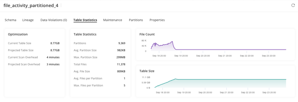
Inspecting the original table, partitioned on the instance_id column, we see that there are  9,369 partitions, created over the 24 hour period. The largest being 300MB and the average size across all remaining partitions is < 1MB. This is expected since the column values are highly unique across our customer base and their varying clusters. 

Ask any data engineering expert and they will tell you that partitioning on such a column is a bad idea. However, this advice goes against the needs of our customer support team that uses this column to quickly root cause customer issues.

Below is a view from Upsolver’s data observability dashboard showing the partitioned table layout and file distribution.

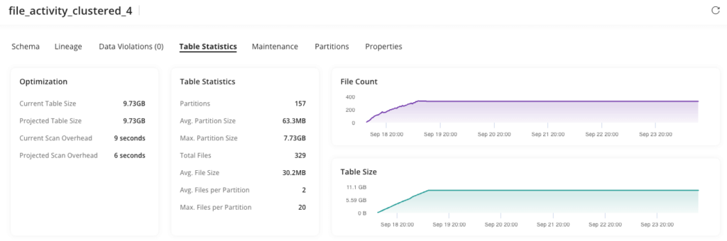
Adaptive Clustering using high cardinality instance_id column

Inspecting the table created using Adaptive Clustering, we can quickly see the difference in partition count and size. The clustered table contains only 157 partitions. The average partition size is a reasonable 63MB. The default partition containing the clustered files comprises 20 compacted and sorted files, averaging around 400MB each (max partition size of 7.7GB / 20 files = ~400MB).

The results: Massive win for ingestion speed and cost savings

These simple tests demonstrate the massive improvement to data ingestion and file maintenance. Adaptive Clustering reduced the total number of partitions by 60X and number of files by 140X without us lifting a finger.

The following table further highlights the write-side improvements. These are key to increase data freshness and reduce overall data ingestion latency and cost.

	Files Ingested	Size reduction	Ingestion Compute (instance hrs)	Ingest time reduction	Compaction Compute (instance hrs)	Optimize time reduction
Partitioned	1.25M	140X	77	8X	416	32X
Clustered	8,852		10		12

In addition to ingestion improvements, Adaptive Clustering accelerated table maintenance tasks such as small file compaction, Iceberg manifest updates and orphan file deletion. These tasks run continuously and are required to maintain highly performant Iceberg tables. The higher the number of partitions and files, the more work the engine needs to perform to compact and manage them, increasing costs dramatically.

Getting Started With Adaptive Clustering

Adaptive Clustering is easy to use and is available free of charge for Upsolver users. Here is how you can get started:

1. Connect your Iceberg catalog like Apache Polaris Catalog or AWS Glue Data Catalog.
2. Create an Iceberg table with the CLUSTER BY keyword to define one or more columns as clustering keys. For example:
   

CREATE ICEBERG TABLE catalog.db.table_name (  c_id BIGINT
  a STRING
  b STRING
) CLUSTER BY c_id;

3. Create an ingestion task to load data into your Iceberg table.

At this point your Iceberg tables are loaded, optimized and accessible from your choice of Iceberg compatible query engine – Snowflake, Amazon Athena and Redshift, Dremio, Trino, Presto, Starrocks, DuckDB, Spark and more.

Adaptive Clustering is the simplest way to partition Iceberg tables

Adaptive Clustering figures out the right data layout for your tables, delivering better write and read performance to manually tuned partitioned tables. It makes it easy for any user to create and load Iceberg tables without planning and testing data layout and partitioning strategies. This enables you to onboard new datasets and make them available to analytics and data science users in minutes without data engineering resources.

Adaptive Clustering is part of Upsolver’s Adaptive Iceberg Optimizer designed to simplify and accelerate creating, managing and using Iceberg tables on Amazon S3 with your favorite query engines. Adaptive Clustering works with Iceberg compatible engines like Snowflake, Amazon Athena and Redshift, Dremio, Starburst, Apache Presto and Trino, DuckDB, ClickHouse, StarRocks and more.

You can get started today for free by signing up to Upsolver or connect with our solution architects to learn more and see how Adaptive Clustering can work for you.